Explain multioutput predictive models with dalex
This notebook provides examples of working with multiclass classification and other multioutput algorithms, e.g. multioutput regression.
A natural example of such an algorithm is a multilayer perceptron neural network.
For a broad overview of the topic, see a comprehensive introduction in the scikit-learn package's documentation: 1.12. Multiclass and multioutput algorithms.
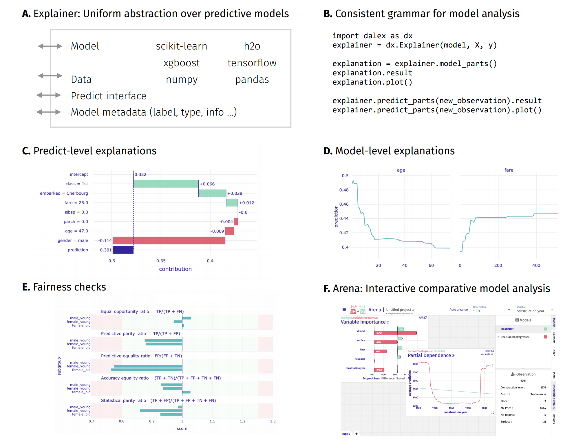
Introduction to dalex: Explanatory Model Analysis: Explore, Explain, and Examine Predictive Models
Imports
import dalex as dx
import numpy as np
import pandas as pd
from sklearn import datasets
from sklearn.ensemble import RandomForestRegressor
from sklearn.multioutput import MultiOutputRegressor
from lightgbm import LGBMClassifier, LGBMRegressor
import plotly
plotly.offline.init_notebook_mode()
import warnings
warnings.filterwarnings('ignore')
dx.__version__
Part 1: treating a multioutput model as multiple singleoutput models
One approach is to use each model's output separately, e.g. the predicted probability for a given class in multiclass classification problem.
Part 1A: Multiclass classification
We will use the iris dataset and the LGBMClassifier model for this example.
# data
X, y = datasets.load_iris(return_X_y=True, as_frame=True)
# model
model = LGBMClassifier(n_estimators=25, verbose=-1)
model.fit(X, y)
# model has 3 outputs
model.predict_proba(X).shape
Let's explain the classification for the first class 0. For that, we need to create a custom predict_function.
# custom (binary) predict function
pf_0 = lambda m, d: m.predict_proba(d)[:, 0]
# custom (binary) target values
y_0 = y == 0
# explainer
exp_0 = dx.Explainer(model, X, y_0, predict_function=pf_0, label="LGBMClassifier: class 0")
exp_0.model_performance()
exp_0.model_parts().plot()
exp_0.model_profile().plot()
Now, let's explain the classification for all the classes. For that, we can loop over multiple explainers.
exp_list = []
for i in range(len(np.unique(y))):
# add i parameter to `predict_function` just to do it in a loop
pf = lambda m, d, i=i: m.predict_proba(d)[:, i]
e = dx.Explainer(
model, X,
y == i,
predict_function=pf,
label=f'LGBMClassifier: class {i}',
verbose=False
)
exp_list += [e]
exp_list
# create multiple explanations
m_profile_list = [e.model_profile() for e in exp_list]
# plot multiple explanations
m_profile_list[0].plot(m_profile_list[1:])
m_parts_list = [e.model_parts() for e in exp_list]
m_parts_list[0].plot(m_parts_list[1:])
We explain predictions in a same way
# choose a data point to explain
observation = X.iloc[[0]]
p_parts_list = [e.predict_parts(observation) for e in exp_list]
p_parts_list[0].plot(p_parts_list[1:], min_max=[-0.1, 1.1])
p_profile_list = [e.predict_profile(observation) for e in exp_list]
p_profile_list[0].plot(p_profile_list[1:])
Part 1B: Multioutput regression
We will use a custom dataset and two models for this example:
RandomForestRegressor, which supports multioutput directly,LGBMRegressorwithMultiOutputRegressor, which involves creating one model for each output independently.
For details, see 1.10.3. Multi-output problems and scikit-learn: Comparing random forests and the multi-output meta estimator.
# create a toy multiregression example
n_outputs = 4
X, y = datasets.make_regression(n_samples=2000, n_features=7, n_informative=5, n_targets=n_outputs, effective_rank=1, noise=0.5, random_state=1)
# summarize the dataset
print(X.shape, y.shape)
# model
model_rf = RandomForestRegressor()
model_rf.fit(X, y)
model_rf.predict(X).shape
The following code returns an error because the LGBMRegressor model does not support multioutput directly.
try:
model_gbm = LGBMRegressor()
model_gbm.fit(X, y)
except Exception as e:
print(f"Error: {e}")
# wrap the second model
model_gbm = MultiOutputRegressor(LGBMRegressor(verbose=-1))
model_gbm.fit(X, y)
model_gbm.predict(X).shape
Like in Part 1A, we explain the regression for all the outputs by looping over multiple explainers.
exp_rf_list, exp_gbm_list = [], []
for i in range(n_outputs):
# add i parameter to `predict_function` just to do it in a loop
pf = lambda m, d, i=i: m.predict(d)[:, i]
e_rf = dx.Explainer(
model_rf, X,
y[:, i],
predict_function=pf,
label=f'RF: output {i}',
verbose=False
)
e_gbm = dx.Explainer(
model_gbm, X,
y[:, i],
predict_function=pf,
label=f'GBM: output {i}',
verbose=False
)
exp_rf_list += [e_rf]
exp_gbm_list += [e_gbm]
exp_rf_list + exp_gbm_list
Let's check the models' performance.
m_performance_list = [e.model_performance() for e in exp_rf_list + exp_gbm_list]
pd.concat([mp.result for mp in m_performance_list], axis=0)
m_performance_list[0].plot(m_performance_list[4:8])
Explain!
m_parts_gbm_list = [e.model_parts(verbose=False) for e in exp_gbm_list]
m_parts_gbm_list[0].plot(m_parts_gbm_list[1::])
If the targets have related values and domains, we could compare their profiles.
m_profile_gbm_list = [e.model_profile(verbose=False) for e in exp_gbm_list]
m_profile_gbm_list[0].plot(m_profile_gbm_list[1::])
Let's compare local explanations.
# choose a data point to explain
observation = X[0, :]
exp_rf_list[1].predict_parts(observation, type="shap").plot(
exp_gbm_list[1].predict_parts(observation, type="shap")
)
Part 2: adapting explanations for multioutput models
Another approach is to customize explanations specifically for multioutput models.
For example, there are loss_functions specific to multiclass classification, which we can substitute when calculating feature importance. We will use the iris dataset and the LGBMClassifier model for this example.
# data
X, y = datasets.load_iris(return_X_y=True, as_frame=True)
# model
model = LGBMClassifier(n_estimators=25, verbose=-1)
model.fit(X, y)
# model has 3 outputs
model.predict_proba(X).shape
# predict function
pf = lambda m, d: m.predict_proba(d)
# explainer
exp = dx.Explainer(model, X, y, predict_function=pf, label="LGBMClassifier: multioutput")
Please note the above warning:
-> residuals : 'residual_function' returns an Error when executed: operands could not be broadcast together with shapes (150,) (150,3)
It is due to the default residual_function expecting predict_function to return a numpy.ndarray (1d). With a wrong predict_function and others, we obtain the following Errors:
try:
exp.model_performance()
except Exception as e:
print(f"Error: {e}")
try:
exp.model_parts()
except Exception as e:
print(f"Error: {e}")
try:
exp.model_profile(verbose=False)
except Exception as e:
print(f"Error: {e}")
Let's define a custom loss_function to work with model_parts, e.g. we can use Cross-entropy loss.
def loss_cross_entropy(y_true, y_pred):
## for loop for code clarity - could be optimized
probs = [0]*len(y_true)
for i, val in enumerate(y_true):
probs[i] = y_pred[i, val]
return np.sum(-np.log(np.maximum(probs, 0.0000001)))
# test if it works
loss_cross_entropy(exp.y, exp.predict(exp.data))
Explain! We obtain one global explanation for the multioutput model.
mp = exp.model_parts(loss_function=loss_cross_entropy)
mp.result
mp.plot()
Let's define a custom residual_function to work with model_diagnostics.
# residual function
def residual_multiclass(model, data, y_true):
# convert target to one-hot encoding
y_true_ohe = np.zeros((len(y_true), max(y_true)+1))
y_true_ohe[np.arange(len(y_true)), y_true] = 1
y_pred = model.predict_proba(data)
# examplary definition of a residual in multiclass
residuals = (y_true_ohe - y_pred).max(axis=1)
return residuals
residual_multiclass(model, X, y)
# explainer
exp_res = dx.Explainer(
model, X, y,
# by default, predict_function needs to return a (1d) numpy.ndarray
predict_function=lambda m, d: m.predict(d),
residual_function=residual_multiclass,
label="LGBMClassifier: multioutput"
)
exp_res.model_diagnostics().plot(variable="petal length (cm)")
Plots
This package uses plotly to render the plots:
- Install extentions to use
plotlyin JupyterLab: Getting Started Troubleshooting - Use
show=Falseparameter inplotmethod to returnplotly Figureobject - It is possible to edit the figures and save them
Resources - https://dalex.drwhy.ai/python
Introduction to the
dalexpackage: Titanic: tutorial and examplesKey features explained: FIFA20: explain default vs tuned model with dalex
How to use dalex with: xgboost, tensorflow, h2o (feat. autokeras, catboost, lightgbm)
Explaining multiclass classification and multioutput regression: Explain multioutput predictive models with dalex
More explanations: residuals, shap, lime
Introduction to the Fairness module in dalex
Introduction to the Aspect module in dalex
Introduction to Arena: interactive dashboard for model analysis
Code in the form of jupyter notebook
Changelog: NEWS
Theoretical introduction to the plots: Explanatory Model Analysis: Explore, Explain, and Examine Predictive Models