Titanic: tutorial and examples

imports

import dalex as dx

import pandas as pd
import numpy as np

from sklearn.neural_network import MLPClassifier
from sklearn.preprocessing import StandardScaler, OneHotEncoder
from sklearn.impute import SimpleImputer
from sklearn.pipeline import Pipeline
from sklearn.compose import ColumnTransformer

import warnings
warnings.filterwarnings('ignore')

import plotly
plotly.offline.init_notebook_mode()

dx.__version__

'1.7.0'

load data

First, divide the data into variables X and a target variable y.

data = dx.datasets.load_titanic()

X = data.drop(columns='survived')
y = data.survived

data.head(10)

	gender	age	class	embarked	fare	sibsp	parch	survived
0	male	42.0	3rd	Southampton	7.1100	0	0	0
1	male	13.0	3rd	Southampton	20.0500	0	2	0
2	male	16.0	3rd	Southampton	20.0500	1	1	0
3	female	39.0	3rd	Southampton	20.0500	1	1	1
4	female	16.0	3rd	Southampton	7.1300	0	0	1
5	male	25.0	3rd	Southampton	7.1300	0	0	1
6	male	30.0	2nd	Cherbourg	24.0000	1	0	0
7	female	28.0	2nd	Cherbourg	24.0000	1	0	1
8	male	27.0	3rd	Cherbourg	18.1509	0	0	1
9	male	20.0	3rd	Southampton	7.1806	0	0	1

create a pipeline model

• numerical_transformer pipeline:

  • numerical_features: choose numerical features to transform
  • impute missing data with median strategy
  • scale numerical features with standard scaler

• categorical_transformer pipeline:

  • categorical_features: choose categorical features to transform
  • impute missing data with 'missing' string
  • encode categorical features with one-hot

• aggregate those two pipelines into a preprocessor using ColumnTransformer

• make a basic classifier model using MLPClassifier - it has 3 hidden layers with sizes 150, 100, 50 respectively

• construct a clf pipeline model, which combines the preprocessor with the basic classifier model

numerical_features = ['age', 'fare', 'sibsp', 'parch']
numerical_transformer = Pipeline(
    steps=[
        ('imputer', SimpleImputer(strategy='median')),
        ('scaler', StandardScaler())
    ]
)

categorical_features = ['gender', 'class', 'embarked']
categorical_transformer = Pipeline(
    steps=[
        ('imputer', SimpleImputer(strategy='constant', fill_value='missing')),
        ('onehot', OneHotEncoder(handle_unknown='ignore'))
    ]
)

preprocessor = ColumnTransformer(
    transformers=[
        ('num', numerical_transformer, numerical_features),
        ('cat', categorical_transformer, categorical_features)
    ]
)

classifier = MLPClassifier(hidden_layer_sizes=(150,100,50), max_iter=500, random_state=0)

clf = Pipeline(steps=[('preprocessor', preprocessor),
                      ('classifier', classifier)])

fit the model

clf.fit(X, y)

Pipeline(steps=[('preprocessor',
                 ColumnTransformer(transformers=[('num',
                                                  Pipeline(steps=[('imputer',
                                                                   SimpleImputer(strategy='median')),
                                                                  ('scaler',
                                                                   StandardScaler())]),
                                                  ['age', 'fare', 'sibsp',
                                                   'parch']),
                                                 ('cat',
                                                  Pipeline(steps=[('imputer',
                                                                   SimpleImputer(fill_value='missing',
                                                                                 strategy='constant')),
                                                                  ('onehot',
                                                                   OneHotEncoder(handle_unknown='ignore'))]),
                                                  ['gender', 'class',
                                                   'embarked'])])),
                ('classifier',
                 MLPClassifier(hidden_layer_sizes=(150, 100, 50), max_iter=500,
                               random_state=0))])

In a Jupyter environment, please rerun this cell to show the HTML representation or trust the notebook.
On GitHub, the HTML representation is unable to render, please try loading this page with nbviewer.org.

create an explainer for the model

exp = dx.Explainer(clf, X, y)

Preparation of a new explainer is initiated

  -> data              : 2207 rows 7 cols
  -> target variable   : Parameter 'y' was a pandas.Series. Converted to a numpy.ndarray.
  -> target variable   : 2207 values
  -> model_class       : sklearn.neural_network._multilayer_perceptron.MLPClassifier (default)
  -> label             : Not specified, model's class short name will be used. (default)
  -> predict function  : <function yhat_proba_default at 0x137744360> will be used (default)
  -> predict function  : Accepts only pandas.DataFrame, numpy.ndarray causes problems.
  -> predicted values  : min = 2.72e-06, mean = 0.337, max = 1.0
  -> model type        : classification will be used (default)
  -> residual function : difference between y and yhat (default)
  -> residuals         : min = -0.921, mean = -0.0146, max = 0.975
  -> model_info        : package sklearn

A new explainer has been created!

introduction to the topic: Explanatory Model Analysis: Explore, Explain, and Examine Predictive Models

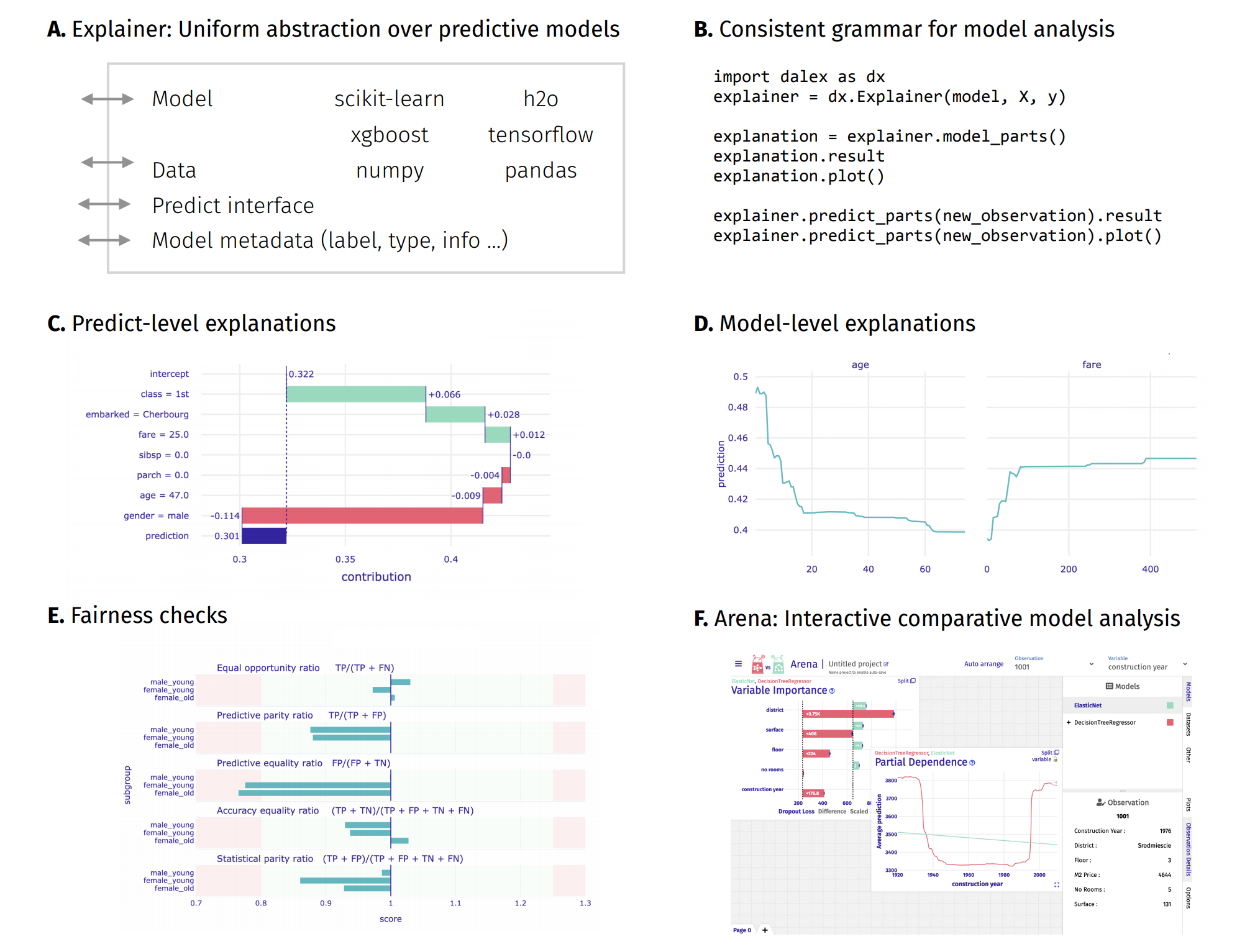
Above functionalities are accessible from the Explainer object through its methods.

Model-level and predict-level methods return a new unique object that contains the result attribute (pandas.DataFrame) and the plot method.

Predict-level explanations

predict

This function is nothing but normal model prediction, however it uses Explainer interface.

Let's create two example persons for this tutorial.

john = pd.DataFrame({'gender': ['male'],
                       'age': [25],
                       'class': ['1st'],
                       'embarked': ['Southampton'],
                       'fare': [72],
                       'sibsp': [0],
                       'parch': 0},
                      index = ['John'])

mary = pd.DataFrame({'gender': ['female'],
                     'age': [35],
                     'class': ['3rd'],
                     'embarked': ['Cherbourg'],
                     'fare': [25],
                     'sibsp': [0],
                     'parch': [0]},
                     index = ['Mary'])

You can make a prediction on many samples at the same time

exp.predict(X)[0:10]

array([0.07907226, 0.20628711, 0.13463174, 0.60372994, 0.76485216,
       0.16150944, 0.03705073, 0.99324938, 0.19563509, 0.12184964])

As well as on only one instance. However, the only accepted format is pandas.DataFrame.

Prediction of survival for John.

exp.predict(john)

array([0.08127727])

Prediction of survival for Mary.

exp.predict(mary)

array([0.8929144])

predict_parts

• 'break_down'

• 'break_down_interactions'

• 'shap'

This function calculates Variable Attributions as Break Down, iBreakDown or Shapley Values explanations.

Model prediction is decomposed into parts that are attributed for particular variables.

bd_john = exp.predict_parts(john, type='break_down', label=john.index[0])
bd_interactions_john = exp.predict_parts(john, type='break_down_interactions', label="John+")

sh_mary = exp.predict_parts(mary, type='shap', B=10, label=mary.index[0])

bd_john.result

	variable_name	variable_value	variable	cumulative	contribution	sign	position	label
0	intercept		intercept	0.336735	0.336735	1.0	8	John
1	class	1st	class = 1st	0.583093	0.246358	1.0	7	John
2	age	25.0	age = 25.0	0.595401	0.012308	1.0	6	John
3	sibsp	0.0	sibsp = 0.0	0.585751	-0.009650	-1.0	5	John
4	fare	72.0	fare = 72.0	0.319029	-0.266722	-1.0	4	John
5	parch	0.0	parch = 0.0	0.300772	-0.018257	-1.0	3	John
6	embarked	Southampton	embarked = Southampton	0.284191	-0.016580	-1.0	2	John
7	gender	male	gender = male	0.081277	-0.202914	-1.0	1	John
8			prediction	0.081277	0.081277	1.0	0	John

bd_john.plot(bd_interactions_john)

sh_mary.result.loc[sh_mary.result.B == 0, ]

	variable	contribution	variable_name	variable_value	sign	label	B
0	gender = female	0.498438	gender	female	1.0	Mary	0
1	embarked = Cherbourg	0.110126	embarked	Cherbourg	1.0	Mary	0
2	class = 3rd	-0.092133	class	3rd	-1.0	Mary	0
3	age = 35.0	0.022643	age	35	1.0	Mary	0
4	sibsp = 0.0	0.016163	sibsp	0	1.0	Mary	0
5	parch = 0.0	0.007954	parch	0	1.0	Mary	0
6	fare = 25.0	-0.007013	fare	25	-1.0	Mary	0

sh_mary.plot(bar_width=16)

exp.predict_parts(john, type='shap', B=10, label=john.index[0]).plot(max_vars=5)

predict_profile

• 'ceteris_paribus'

This function computes individual profiles aka Ceteris Paribus Profiles.

cp_mary = exp.predict_profile(mary, label=mary.index[0])
cp_john = exp.predict_profile(john, label=john.index[0])

cp_mary.result.head()

Calculating ceteris paribus: 100%|██████████| 7/7 [00:00<00:00, 106.99it/s]
Calculating ceteris paribus: 100%|██████████| 7/7 [00:00<00:00, 69.35it/s]

	gender	age	class	embarked	fare	sibsp	parch	_original_	_yhat_	_vname_	_ids_	_label_
Mary	male	35.000000	3rd	Cherbourg	25.0	0.0	0.0	female	0.129222	gender	Mary	Mary
Mary	female	35.000000	3rd	Cherbourg	25.0	0.0	0.0	female	0.892914	gender	Mary	Mary
Mary	female	0.166667	3rd	Cherbourg	25.0	0.0	0.0	35	0.992733	age	Mary	Mary
Mary	female	0.905000	3rd	Cherbourg	25.0	0.0	0.0	35	0.991484	age	Mary	Mary
Mary	female	1.643333	3rd	Cherbourg	25.0	0.0	0.0	35	0.990023	age	Mary	Mary

cp_mary.plot(cp_john)

cp_john.plot(cp_mary, variable_type = "categorical")

Model-level explanations

model_performance

• 'classification'

• 'regression'

This function calculates various Model Performance measures:

• classification: F1, accuracy, recall, precision and AUC
• regression: mean squared error, R squared, median absolute deviation

mp = exp.model_performance(model_type = 'classification')
mp.result

	recall	precision	f1	accuracy	auc
MLPClassifier	0.651195	0.813708	0.723437	0.839601	0.877305

mp.result.auc[0]

0.877305256586716

mp.plot(geom="roc")

model_parts

• 'variable_importance'

• 'ratio'

• 'difference'

This function calculates Variable Importance.

vi = exp.model_parts()
vi.result

	variable	dropout_loss	label
0	_full_model_	0.116292	MLPClassifier
1	parch	0.144645	MLPClassifier
2	fare	0.147404	MLPClassifier
3	sibsp	0.154644	MLPClassifier
4	embarked	0.158866	MLPClassifier
5	age	0.204129	MLPClassifier
6	class	0.242640	MLPClassifier
7	gender	0.371637	MLPClassifier
8	_baseline_	0.499977	MLPClassifier

vi.plot(max_vars=5)

There is also a possibility of calculating variable importance of group of variables.

vi_grouped = exp.model_parts(variable_groups={'personal': ['gender', 'age', 'sibsp', 'parch'],
                                     'wealth': ['class', 'fare']})
vi_grouped.result

	variable	dropout_loss	label
0	_full_model_	0.125230	MLPClassifier
1	wealth	0.260403	MLPClassifier
2	personal	0.471375	MLPClassifier
3	_baseline_	0.499360	MLPClassifier

vi_grouped.plot()

model_profile

• 'partial'

• 'accumulated'

This function calculates explanations that explore model response as a function of selected variables.

The explanations can be calulated as Partial Dependence Profile or Accumulated Local Dependence Profile.

pdp_num = exp.model_profile(type = 'partial', label="pdp")

Calculating ceteris paribus: 100%|██████████| 7/7 [00:00<00:00, 20.98it/s]

ale_num = exp.model_profile(type = 'accumulated', label="ale")

Calculating ceteris paribus: 100%|██████████| 7/7 [00:00<00:00, 26.08it/s]
Calculating accumulated dependency: 100%|██████████| 4/4 [00:00<00:00, 21.89it/s]

pdp_num.plot(ale_num)

pdp_cat = exp.model_profile(type = 'partial', variable_type='categorical',
                            variables = ["gender","class"], label="pdp")

ale_cat = exp.model_profile(type = 'accumulated', variable_type='categorical',
                            variables = ["gender","class"], label="ale")

Calculating ceteris paribus: 100%|██████████| 2/2 [00:00<00:00, 98.22it/s]
Calculating ceteris paribus: 100%|██████████| 2/2 [00:00<00:00, 126.33it/s]
Calculating accumulated dependency: 100%|██████████| 2/2 [00:00<00:00, 42.48it/s]

ale_cat.plot(pdp_cat)

Hover over all of the above plots for tooltips with more information.

Saving and loading Explainers

You can easily save an Explainer to the pickle (or generaly binary form) and load it again. Any local or lambda function in the Explainer object will be dropped during saving. Residual function by default is local, thus, if default, it is always dropped. Default functions can be retrieved during loading.

# this converts explainer to a binary form
# exp.dumps()

# this load explainer again
# dx.Explainer.loads(pickled)

# this will not retrieve default function if dropped
# dx.Explainer.loads(pickled, use_defaults=False)

# this will save your explainer to the file
# with open('explainer.pkl', 'wb') as fd:
#     exp.dump(fd)

# this will load your explainer from the file
# with open('explainer.pkl', 'rb') as fd:
#     dx.Explainer.load(fd)

Plots

This package uses plotly to render the plots:

• Install extentions to use plotly in JupyterLab: Getting Started Troubleshooting
• Use show=False parameter in plot method to return plotly Figure object
• It is possible to edit the figures and save them

Resources - https://dalex.drwhy.ai/python

• Introduction to the dalex package: Titanic: tutorial and examples

• Key features explained: FIFA20: explain default vs tuned model with dalex

• How to use dalex with: xgboost, tensorflow, h2o (feat. autokeras, catboost, lightgbm)

• More explanations: residuals, shap, lime

• Introduction to the Fairness module in dalex

• Introduction to the Aspect module in dalex

• Introduction to Arena: interactive dashboard for model exploration

• Code in the form of jupyter notebook

• Changelog: NEWS

• Theoretical introduction to the plots: Explanatory Model Analysis: Explore, Explain, and Examine Predictive Models