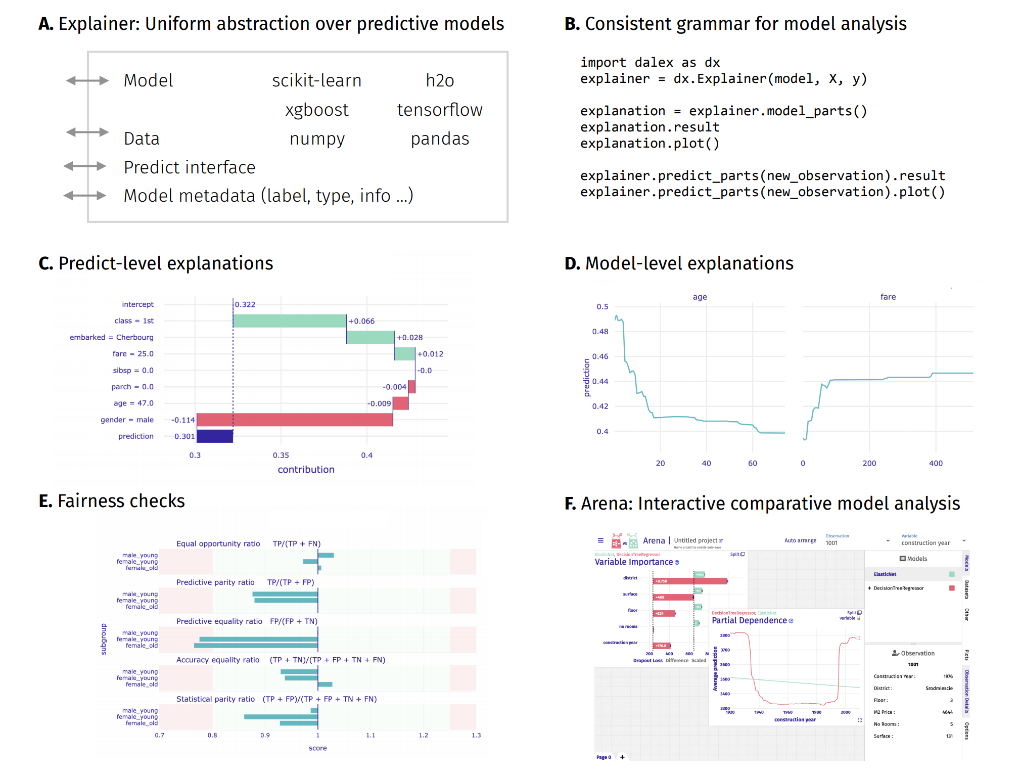
tensorflow + dalex = :)
introduction to the topic: Explanatory Model Analysis: Explore, Explain, and Examine Predictive Models
In [1]:
import warnings
warnings.filterwarnings('ignore')

import plotly
plotly.offline.init_notebook_mode()
read data
In [2]:
import pandas as pd
pd.__version__
Out[2]:
In [3]:
data = pd.read_csv("https://raw.githubusercontent.com/pbiecek/xai-happiness/main/happiness.csv", index_col=0)
data.head()
Out[3]:
In [4]:
X, y = data.drop('score', axis=1), data.score
n, p = X.shape
create a model
In [5]:
import tensorflow as tf
tf.__version__
Out[5]:
In [6]:
tf.random.set_seed(11)

normalizer  = tf.keras.layers.Normalization(input_shape=[p,])
normalizer.adapt(X.to_numpy())

model = tf.keras.Sequential([
    normalizer,
    tf.keras.layers.Dense(p*2, activation='relu'),
    tf.keras.layers.Dense(p*3, activation='relu'),
    tf.keras.layers.Dense(p*2, activation='relu'),
    tf.keras.layers.Dense(p, activation='relu'),
    tf.keras.layers.Dense(1, activation='linear')
])

model.compile(
    optimizer=tf.keras.optimizers.Adam(0.001),
    loss=tf.keras.losses.mae
)
In [7]:
model.fit(X, y, batch_size=int(n/10), epochs=2000, verbose=False)
Out[7]:
explain the model
Explainer initialization communicates useful information
In [8]:
import dalex as dx
dx.__version__
Out[8]:
In [9]:
explainer = dx.Explainer(model, X, y, label='happiness')
model level explanations
firstly, assess the model fit to training data
In [10]:
explainer.model_performance()
Out[10]:
which features are the most important?
In [11]:
explainer.model_parts().plot()
what are the continuous relationships between variables and predictions?
In [12]:
explainer.model_profile().plot(variables=['social_support', 'healthy_life_expectancy',
                                          'gdp_per_capita', 'freedom_to_make_life_choices'])
what about residuals?
In [13]:
explainer.model_diagnostics().plot(variable='social_support', yvariable="abs_residuals", marker_size=5, line_width=3)
In [14]:
explainer.model_diagnostics().result
Out[14]:
predict level explanations
investigate the specific country
In [15]:
explainer.predict_parts(X.loc['Poland'], type='shap').plot()
or several countries
In [16]:
pp_list = []
for country in ['Afghanistan', 'Belgium', 'China', 'Denmark', 'Ethiopia']:
    pp = explainer.predict_parts(X.loc[country], type='break_down')
    pp.result.label = country
    pp_list += [pp]
pp_list[0].plot(pp_list[1::], min_max=[2.5, 8.5])
surrogate approximation
In [17]:
lime_explanation = explainer.predict_surrogate(X.loc['United States'], mode='regression')
In [18]:
lime_explanation.plot()

In [19]:
lime_explanation.result
Out[19]:
interpretable surrogate model
In [20]:
surrogate_model = explainer.model_surrogate(max_vars=4, max_depth=3)
surrogate_model.performance
Out[20]:
In [21]:
surrogate_model.plot()

Plots
This package uses plotly to render the plots:
- Install extentions to use
plotlyin JupyterLab: Getting Started Troubleshooting - Use
show=Falseparameter inplotmethod to returnplotly Figureobject - It is possible to edit the figures and save them
Resources - https://dalex.drwhy.ai/python
Introduction to the
dalexpackage: Titanic: tutorial and examplesKey features explained: FIFA20: explain default vs tuned model with dalex
How to use dalex with: xgboost, tensorflow, h2o (feat. autokeras, catboost, lightgbm)
More explanations: residuals, shap, lime
Introduction to the Fairness module in dalex
Introduction to the Aspect module in dalex
Introduction to Arena: interactive dashboard for model exploration
Code in the form of jupyter notebook
Changelog: NEWS
Theoretical introduction to the plots: Explanatory Model Analysis: Explore, Explain, and Examine Predictive Models