FIFA 20: explain default vs tuned model with dalex
imports
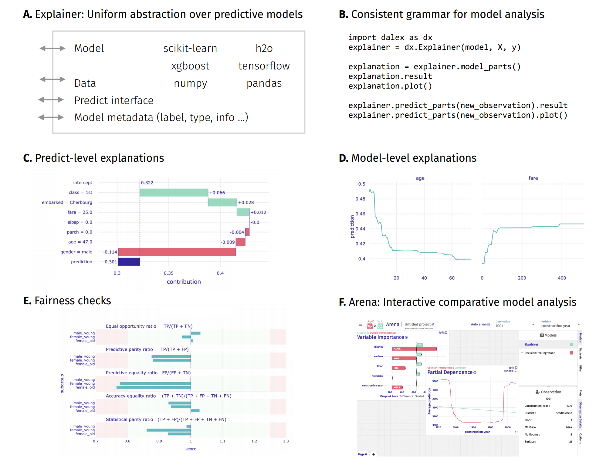
import dalex as dx

import numpy as np
import pandas as pd

from lightgbm import LGBMRegressor
from sklearn.model_selection import train_test_split
from sklearn.model_selection import RandomizedSearchCV

import warnings
warnings.filterwarnings('ignore')

import plotly
plotly.offline.init_notebook_mode()
dx.__version__
load data
Load fifa, the preprocessed players_20 dataset. It contains 5000 'overall' best players and 43 columns. These are:
- short_name (index)
- nationality of the player (not used in modeling)
- overall, potential, value_eur, wage_eur (4 potential target variables)
- age, height, weight, attacking skills, defending skills, goalkeeping skills (37 variables)
It is advised to leave only one target variable for modeling.
data = dx.datasets.load_fifa()
data.head(10)
Divide the data into variables X and a target variable y. Here we will be predicting the value of the best players.
X = data.drop(["nationality", "overall", "potential", "value_eur", "wage_eur"], axis = 1)
y = data['value_eur']
The target variable is skewed so we transform it with log for a better fit.
ylog = np.log(y)

import matplotlib.pyplot as plt
plt.hist(ylog, bins='auto')
plt.title("ln(value_eur)")
plt.show()

Split the data into train and test.
X_train, X_test, ylog_train, ylog_test, y_train, y_test = \
    train_test_split(X, ylog, y, test_size=0.25, random_state=4)
create a default boosting model
gbm_default = LGBMRegressor()

gbm_default.fit(X_train, ylog_train)
create a tuned model
gbm_default._estimator_type
#:# hp tuning
estimator = LGBMRegressor(n_jobs = -1)
param_test = {
    'n_estimators': list(range(201,1202,50)),
    'num_leaves': list(range(6, 42, 5)),
    'min_child_weight': [1e-3, 1e-2, 1e-1, 15e-2],
    'learning_rate': [1e-3, 1e-2, 1e-1, 15e-2]
}

rs = RandomizedSearchCV(
    estimator=estimator,
    param_distributions=param_test,
    n_iter=100,
    cv=4,
    random_state=1
)

# rs.fit(X, ylog)
# print('Best score reached: {} with params: {} '.format(rs.best_score_, rs.best_params_))
#:# best parameters after 100 iterations
best_params = {'num_leaves': 6,
               'n_estimators': 951,
               'min_child_weight': 0.1,
               'learning_rate': 0.15}
gbm_tuned = LGBMRegressor(**best_params)
gbm_tuned.fit(X_train, ylog_train)
create explainers for the models
We aim to see real values of the target variable in the explanations (not log). Therefore, we need to make a custom predict_function.
def predict_function(model, data):
    return np.exp(model.predict(data))
exp_default = dx.Explainer(gbm_default, X_test, y_test,
                           predict_function=predict_function, label='default')
exp_tuned = dx.Explainer(gbm_tuned, X_test, y_test,
                         predict_function=predict_function, label='tuned')
introduction to the topic: Explanatory Model Analysis: Explore, Explain, and Examine Predictive Models
Above functionalities are accessible from the Explainer object through its methods.
Model-level and predict-level methods return a new unique object that contains the result attribute (pandas.DataFrame) and the plot method.
mp_default = exp_default.model_performance("regression")
mp_default.result
mp_tuned = exp_tuned.model_performance("regression")
mp_tuned.result
mp_default.plot(mp_tuned)
This are very big values so the difference on paper may be very subtle.
What are the differences between these two models? Let's find out.
Customize the computation with parameters:
loss_function function to use for drop-out loss evaluation
B number of bootstrap rounds (e.g.
15for slower computation but more stable results)N number of observations to use (e.g.
500for faster computation but less stable results)variable_groups Dict of lists of variables. Each list is treated as one group. This is for testing joint variable importance
X.columns
variable_groups = {
    'age': ['age'],
    'body': ['height_cm', 'weight_kg'],
    'attacking': ['attacking_crossing',
       'attacking_finishing', 'attacking_heading_accuracy',
       'attacking_short_passing', 'attacking_volleys'],
    'skill': ['skill_dribbling',
       'skill_curve', 'skill_fk_accuracy', 'skill_long_passing',
       'skill_ball_control'],
    'movement': ['movement_acceleration', 'movement_sprint_speed',
       'movement_agility', 'movement_reactions', 'movement_balance'],
    'power': ['power_shot_power', 'power_jumping', 'power_stamina', 'power_strength',
       'power_long_shots'],
    'mentality': ['mentality_aggression', 'mentality_interceptions',
       'mentality_positioning', 'mentality_vision', 'mentality_penalties',
       'mentality_composure'],
    'defending': ['defending_marking', 'defending_standing_tackle',
       'defending_sliding_tackle'],
    'goalkeeping' : ['goalkeeping_diving',
       'goalkeeping_handling', 'goalkeeping_kicking',
       'goalkeeping_positioning', 'goalkeeping_reflexes']
}
vi_default = exp_default.model_parts(variable_groups=variable_groups, B=15, random_state=0)
vi_tuned = exp_tuned.model_parts(variable_groups=variable_groups, B=15)
Customize the plot with parameters:
vertical_spacing value between
0.0and1.0(e.g.0.15for more space between the plots)rounding_function rounds the contributions (e.g.
np.round,np.rint,np.ceil)digits (e.g.
2fornp.round,Nonefornp.rint)
vi_default.plot(vi_tuned,
                max_vars=6, rounding_function=np.rint, digits=None, vertical_spacing=0.15)
Variables connected with body and power aren't important for these models. It is also true for goalkeeping. This might mean that goalkeepers predictions aren't accurate. The most important factors in predicting players value are skill, attacking and movement.
It seems like the default model is focusing on movement variables too much and doesn't find other variables so important, especially skill. The tuned model finds mentality and defending quite important. Next, we will examine these variables closer.
Aggregated Profiles
Choose a proper algorithm. The explanations can be calulated as Partial Dependence Profile or Accumulated Local Dependence Profile.
The key parameter is N number of observations to use (e.g. 800 for slower computation but more stable results).
Here we will use ale plots, which work better if the explanatory variables are correlated.
ale_default = exp_default.model_profile(type = 'accumulated', N=800, label='ale-default')
ale_tuned = exp_tuned.model_profile(type = 'accumulated', N=800, label='ale-tuned')
ale_default.plot(ale_tuned, variables = ['goalkeeping_positioning', 'power_stamina',
                                           'mentality_vision', 'defending_marking',
                                           'attacking_finishing', 'attacking_heading_accuracy',
                                           'attacking_short_passing', 'skill_ball_control'])
Overall, we can see that the tuned model is using more variables. Examples are defending_marking, goalkeeping_positioning, mentality_vision, power_stamina, skill_ball_control and attacking variables.
It also acts differently with variables like age and movement_reactions.
ale_default.plot(ale_tuned, variables = ['age', 'movement_reactions'])
Variable Attribution
Choose a proper algorithm. The explanations can be calulated as Break Down, iBreakDown or Shapley Values.
For type='shap' the key parameter is B number of bootstrap rounds (e.g. 10 for faster computation but less stable results).
Let's find out what attributes to the value of the best players.
va = {'ibd':[], 'sh':[]}

for name in data.index[0:3]:
    player = X.loc[name,]

    ibd = exp_tuned.predict_parts(player, type='break_down_interactions', label=name)
    sh = exp_tuned.predict_parts(player, type='shap', B=10, label=name)

    va['ibd'].append(ibd)
    va['sh'].append(sh)
va['ibd'][0].plot(va['ibd'][1:3],
                  rounding_function=lambda x, digits: np.rint(x, digits).astype(int),
                  digits=None, max_vars=10)
va['sh'][0].plot(va['sh'][1:3],
                 rounding_function=lambda x, digits: np.rint(x, digits).astype(int),
                 digits=None, max_vars=10)
Looking at the Break Down plots, age and movement_ractions variables are standing out. Let's focus on them more.
cp = exp_tuned.predict_profile(X.iloc[2:3,],
                               variables=['age', 'movement_reactions'],
                               label=X.index[2]) # variables to calculate
cp.plot(size=3, title="What If? Neymar Jr") # larger width of the line and dot size & change title
Here we see how the prediction would change if Neymar Jr was younger/older or had lower movement_reactions.
Hover over all of the above plots for tooltips with more information.
Plots
This package uses plotly to render the plots:
- Install extentions to use
plotlyin JupyterLab: Getting Started Troubleshooting - Use
show=Falseparameter inplotmethod to returnplotly Figureobject - It is possible to edit the figures and save them
Resources - https://dalex.drwhy.ai/python
Introduction to the
dalexpackage: Titanic: tutorial and examplesKey features explained: FIFA20: explain default vs tuned model with dalex
How to use dalex with: xgboost, tensorflow, h2o (feat. autokeras, catboost, lightgbm)
More explanations: residuals, shap, lime
Introduction to the Fairness module in dalex
Introduction to the Aspect module in dalex
Introduction to Arena: interactive dashboard for model exploration
Code in the form of jupyter notebook
Changelog: NEWS
Theoretical introduction to the plots: Explanatory Model Analysis: Explore, Explain, and Examine Predictive Models